Following are 3 different ways to segregate Positive and Negative values from list of numbers in Excel.
Table of Contents
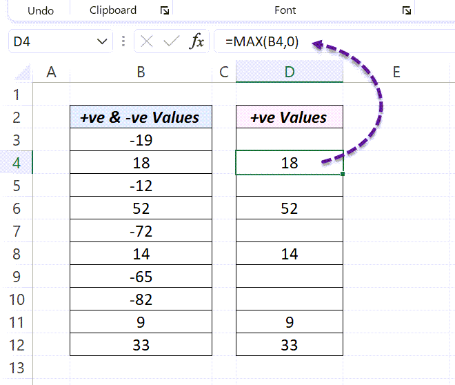
MAX and MIN Function to separate Positive and Negative values
The MAX function in Excel will return the largest among 2 or more numbers supplied into it. This property of MAX function is used below to check whether a number is positive or not and extract it accordingly.
=MAX(B4,0) will return Zero, if the value in the cell B4 is less than Zero and will the return number itself, if the value is greater than Zero.
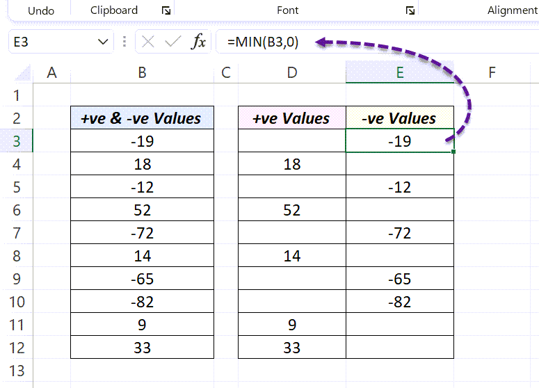
Similarly, the MIN function can be used to extract negative numbers.
=MIN(B3,0)
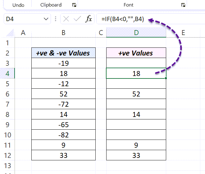
IF Function to separate Positive and Negative values
Using the IF function we can check whether a number is greater than Zero or not and return it accordingly.
=IF(B4<0,"",B4)
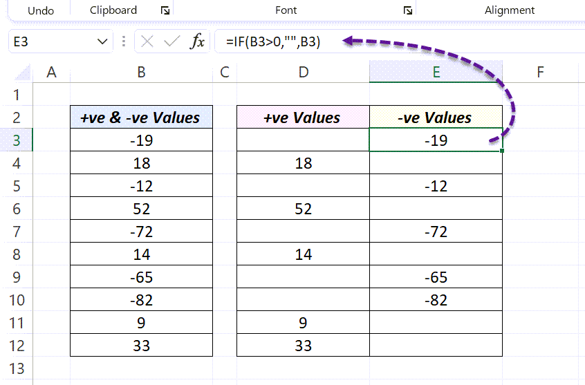
Same technique used to extract negative numbers.
=IF(B3>0,"",B3)
Power Query to separate Positive and Negative values
To extract Positive and Negative numbers into separate columns using Power Query,
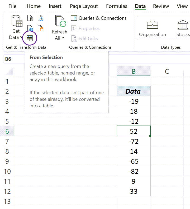
Select the Table containing numbers > go to the Data tab of the Excel ribbon and click on From Selection
If the table containing data isn’t an official Excel table, we will be prompted to convert the data range into an Excel table.
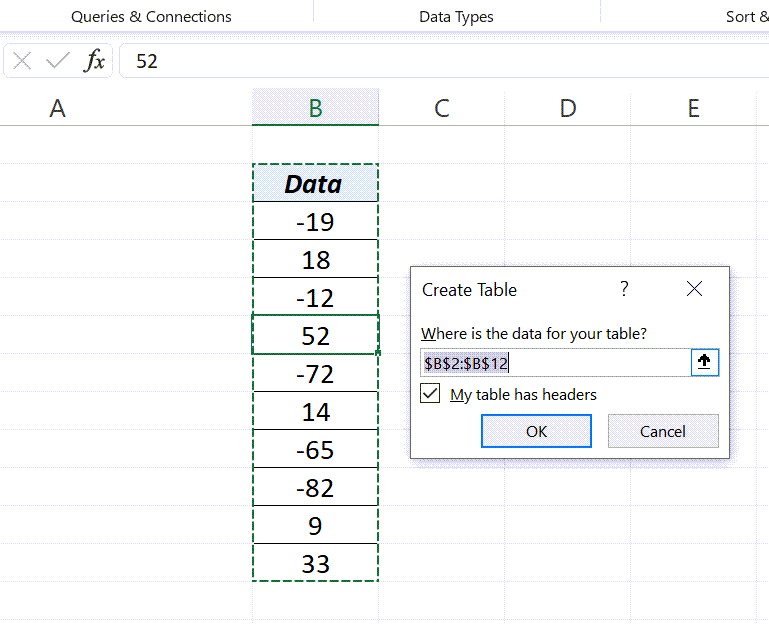
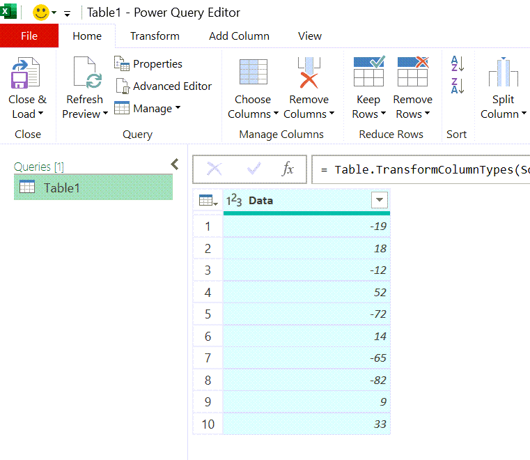
Click OK and the selected table will be loaded into the Power Query Editor of Excel.
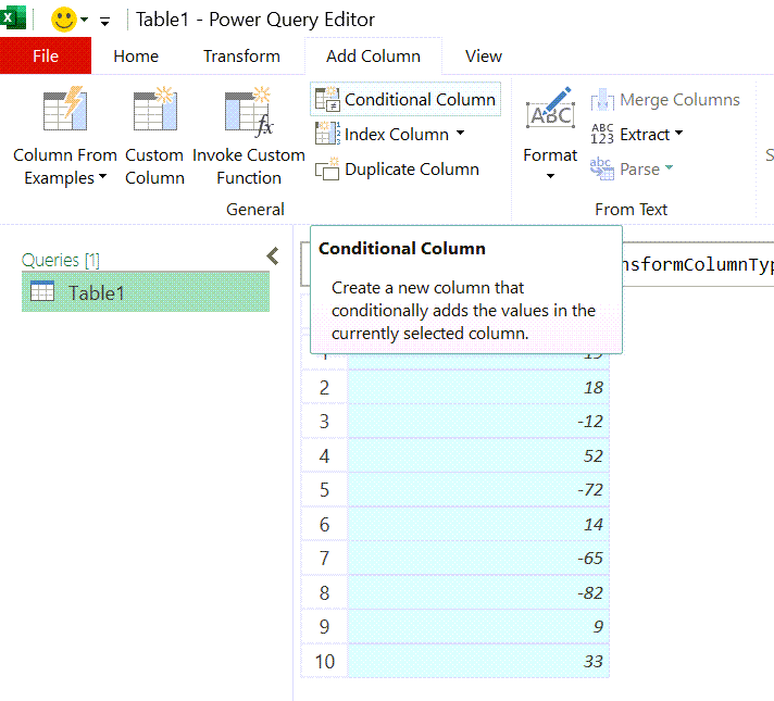
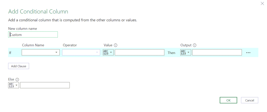
To extract the positive numbers into a new column, go to the Add Column tab of the Power Query Editor > click on Conditional Column
A dialog called Add Conditional Column will be activated. In the dialog we have to define 6 values.
New column name – Positive
Column Name – Data, the column containing values
Operator – is greater than
Value – 0
Output – Here we have two options, Enter a value and Select a column. Choose the second option and select the column called Data.
Else – use the Space character
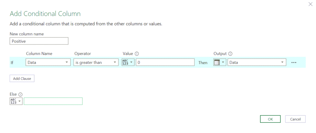
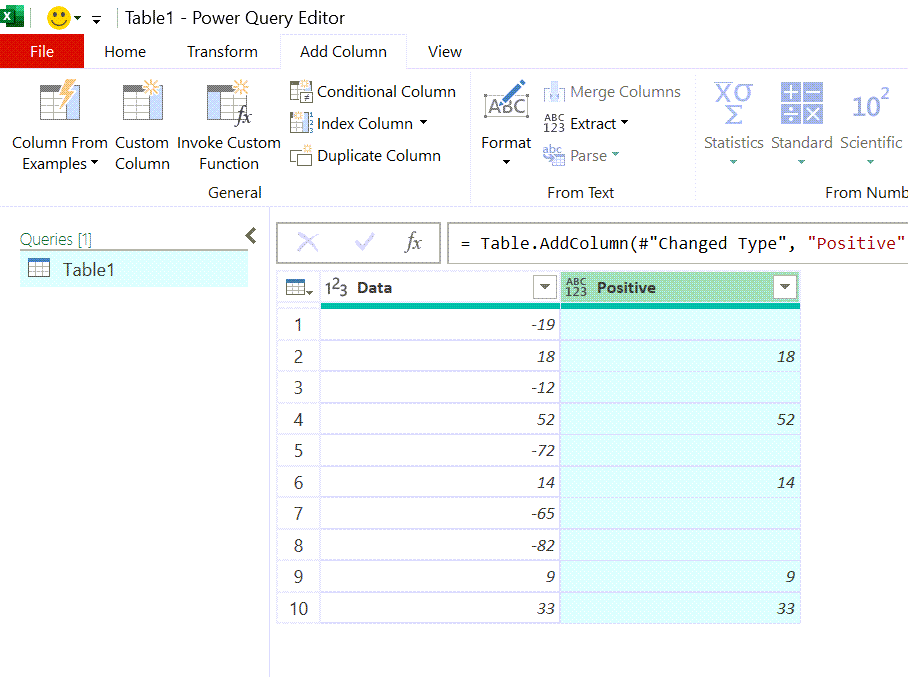
Click on OK and we have a new column called Positive containing positive values in it.
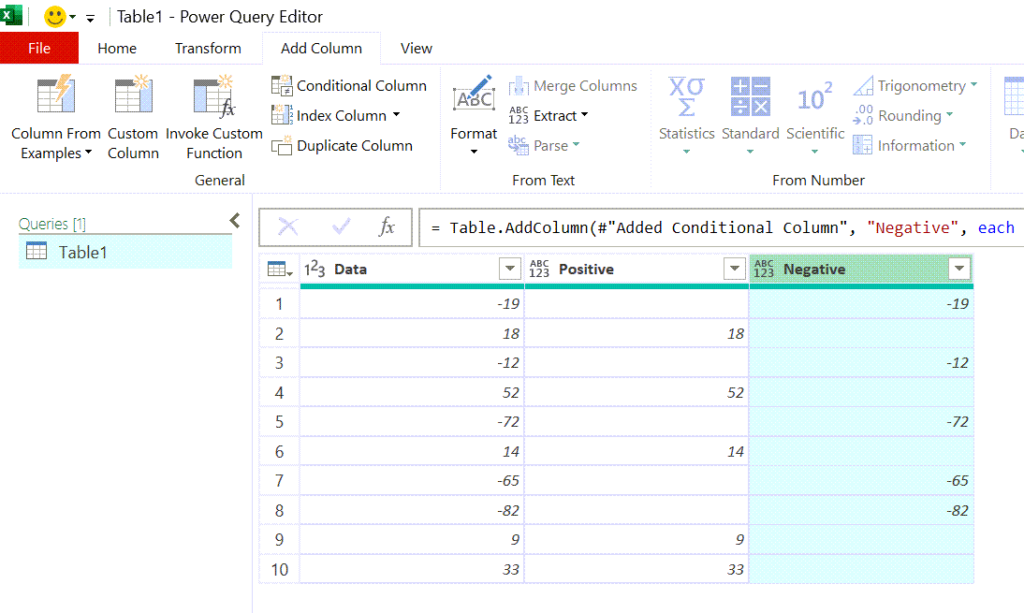
Once again activate the Add Conditional Column dialog and define the parameters to extract the Negative numbers.
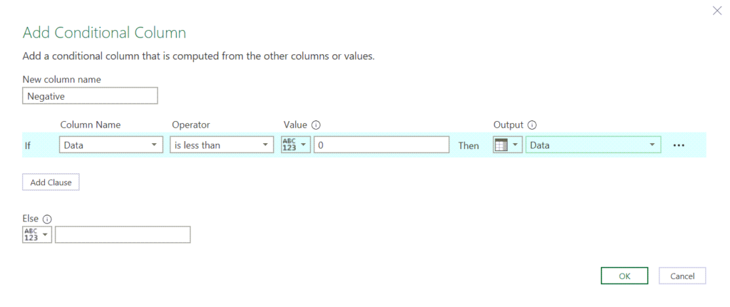
Click on OK and we have a new column called Negative containing the negative values in it.
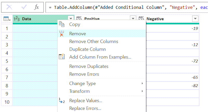
Before loading this data into the Excel worksheet, let’s remove the column called Data. For that right-click on the column header and select Remove.
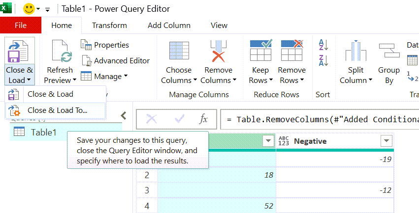
Now to load this data into our Excel worksheet, Click on the split button called Close & Load in the Home tab of the Power Query Editor > Close and Load to…
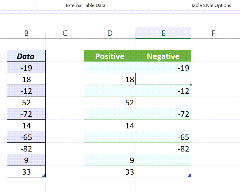
A dialog called Import Data will be activated. Using this dialog, specify the location where you want to insert the output table and click on OK.
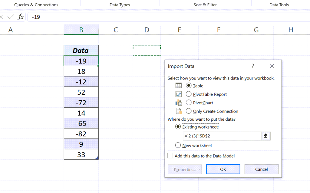
And we have a table with Positive and Negative values in two separate columns.
Add a few Positive and Negative values to the source table and click on the Refresh button in the Data tab to see the dynamic nature of this method.