In this blog post, I will show you how to hide the formulas used in an Excel Worksheet and display only the results of those formulas.
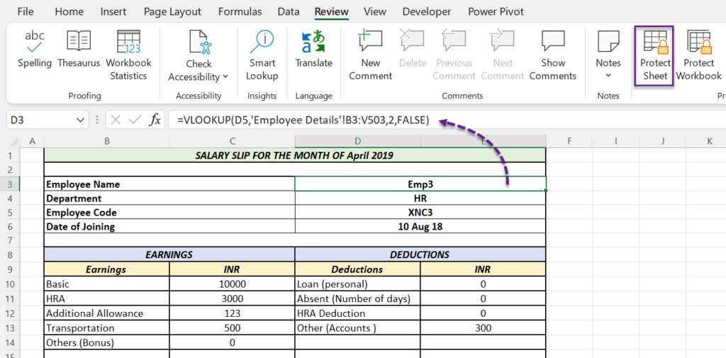
Following is an Excel Worksheet used by a H.R Manager, for generating the Payslips of his colleagues.
Before sharing this workbook with other executives, the H.R manager wants to hide the formulas used in the Worksheet. He also want to restrict the users from modifying the content of his Worksheet.
Here is how he can accomplish this task.
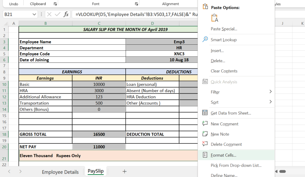
Select all those cells containing formulas > right-click > Format Cells…
in the Format Cells dialog > go to the Protection tab > mark the checkbox against Hidden and Click on OK.
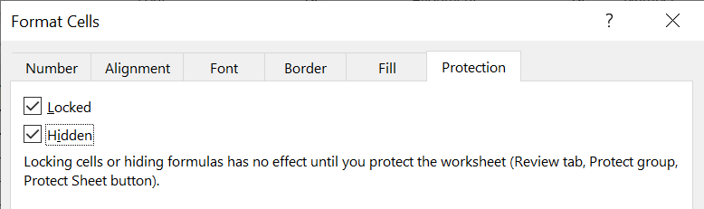
Note: By default, the checkbox for Locked will marked. If not, mark that too.
As you can read from the Format Cells dialog, Locking cells or hiding formulas has no effect until we protect the Worksheet.
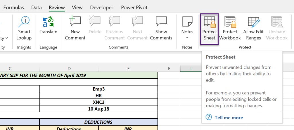
So to protect the worksheet, go to the Review tab of the Excel ribbon > click on Protect Sheet
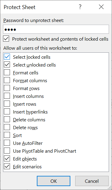
In the dialog called Protect Sheet, type in a Password and Click OK
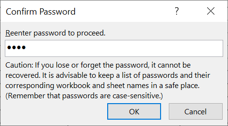
Reenter the Password and Click OK to confirm the Password.
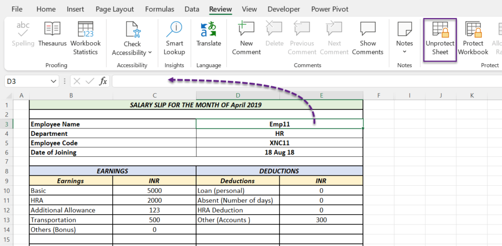
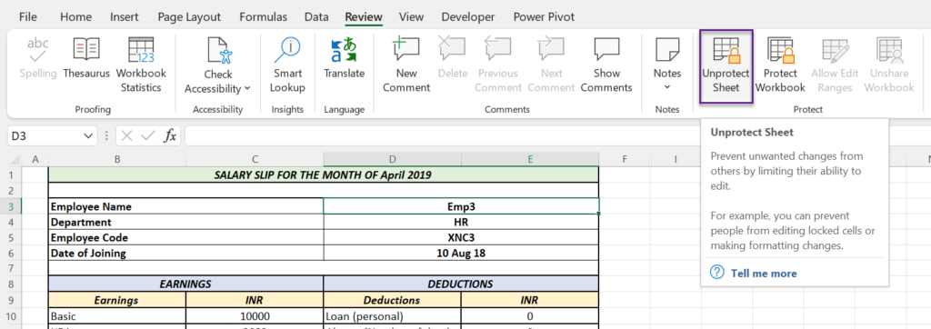
The Protect Sheet button will be replaced with Unprotect Sheet, indicating that you are on a protected sheet.
Now that we have ‘locked the cells and protected the worksheet’, check the cells containing formula.
The formula bar will appear blank.
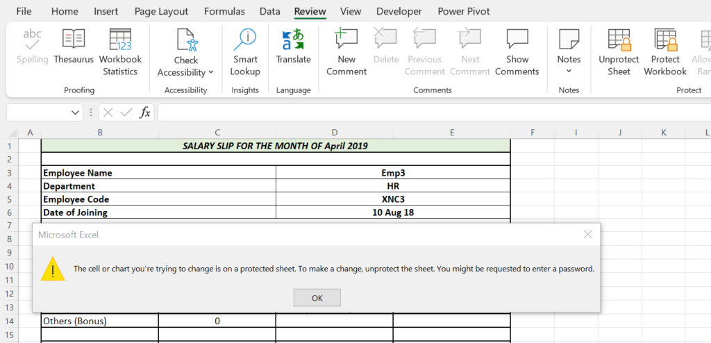
And whenever you try to modify a locked cell on a protected worksheet, Excel will display a warning message.
To remove protection, click on Unprotect Sheet in the Review tab.
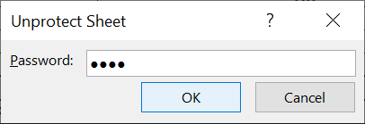
A dialog called Unprotect Sheet will be activated. Type in the Password and click OK.
Now that the protection has been removed, check the cells with formula and you can see the formula in the formula bar.