This Excel tutorial is about 3 different methods to find the common values between two Lists or Tables in Excel.
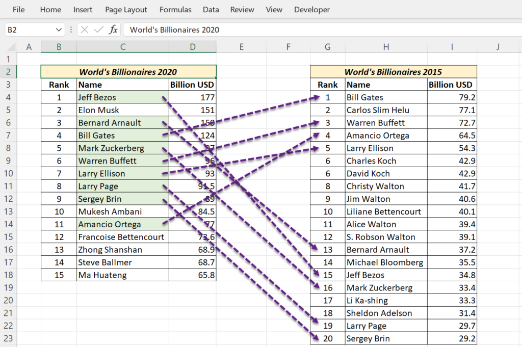
Here we have 2 lists of World’s Billionaires, one from the year 2015 and other one from 2020.
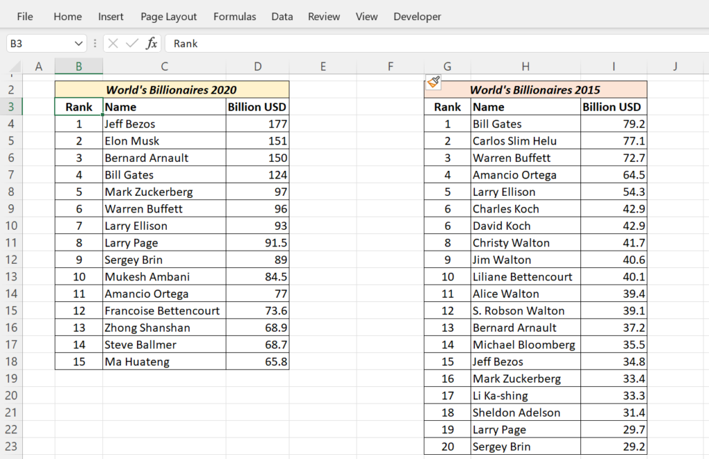
Following are different methods to find the Names that are present in both lists.
Table of Contents
MATCH function to find common values
The MATCH function and many other Lookup functions in Excel can be used to check whether a particular value is present in a list or not. Here, I have used the following formula to compare each name of first list with the second list.
=MATCH(C4,$H$4:$H$23,0)
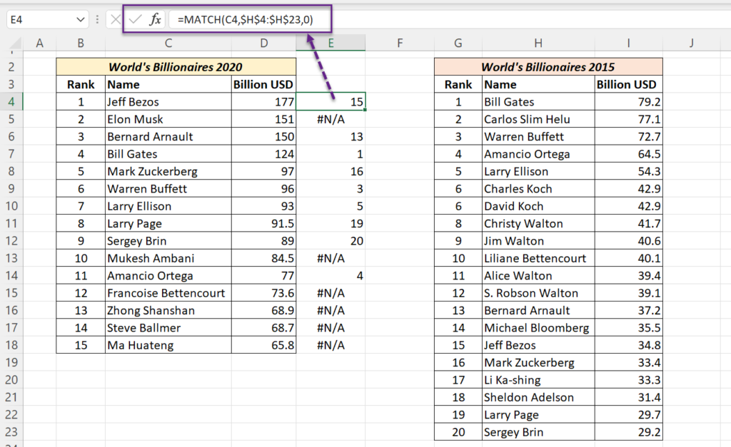
Whenever MATCH function finds a match, it will return the position of the matching value in the second list, otherwise a #N/A Error.
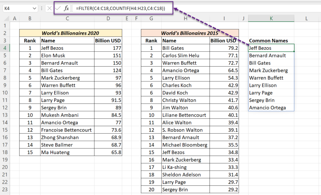
If you want to extract the common values, use the FILTER function.
=FILTER(C4:C18,COUNTIF(H4:H23,C4:C18))
Conditional Formatting to find common values
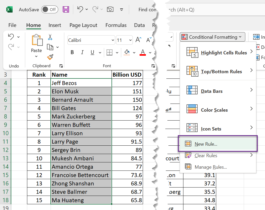
The same formula which we used to spot the common values can be combined with Conditional Formatting to highlight the cells containing common values.
To highlight cells with common values, select the cells containing names > in the Home tab > Conditional Formatting > New Rule…
A dialog called New Formatting Rule will be activated. Select ‘Use a formula to determine which cells to format’ and type in the following formula.
=ISNUMBER(MATCH($C4,$H$4:$H$23,0))
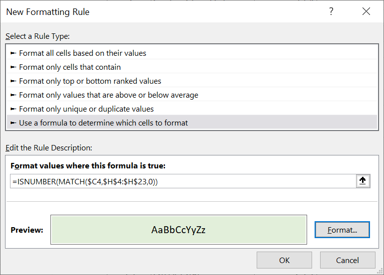
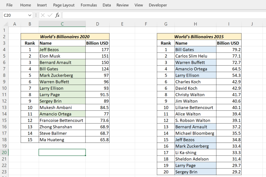
Click on the Format button and define the formatting to be applied for cells with common values. Here, I have selected light Green color so that the cells will be highlighted in that color.
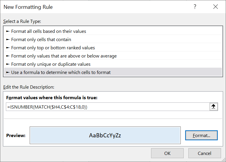
To highlight common values in the second list (data range H4:H23), use the following formula with Conditional Formatting.
=ISNUMBER(MATCH($H4,C$4:C$18,0))
The cells with common values are highlighted in light Blue color.
Power Query to find common records
Now, the Power Query method to find the common values between two lists.
First of all we have to convert both the Lists or Tables into official Excel Tables and load them individually into the Power Query Editor of Excel.
To load a Table into the Power Query Editor, Select the Table > go to the Data tab of the Excel Ribbon > in the category Get & Transform Data, click on From Selection
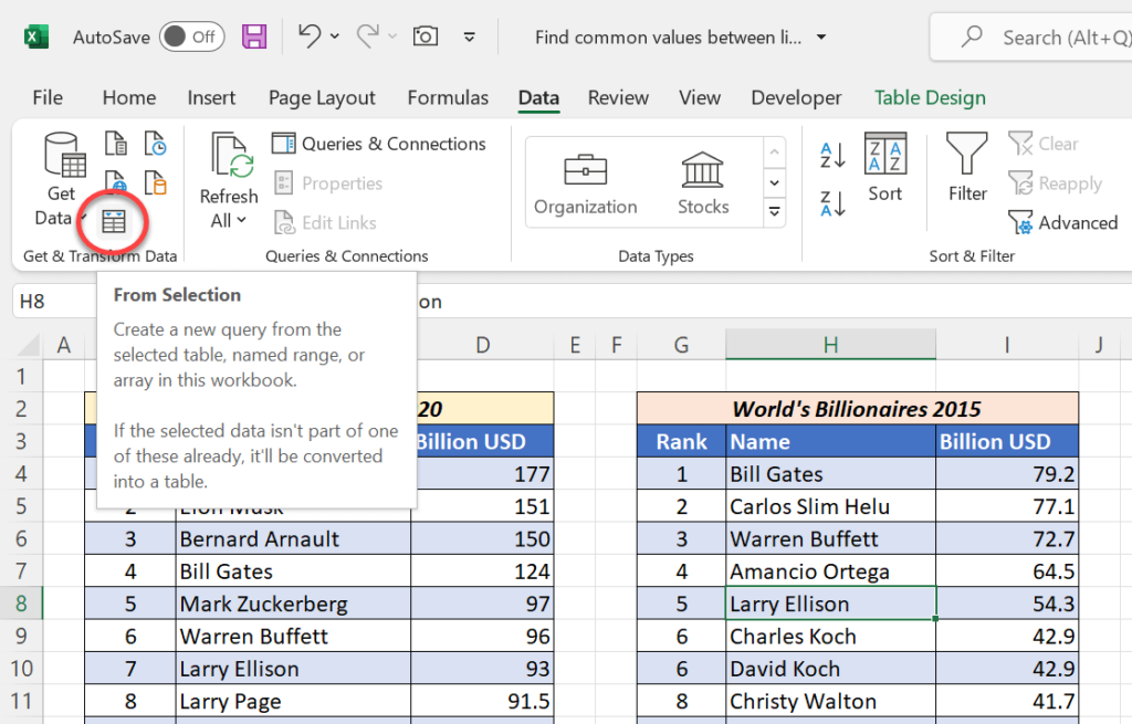
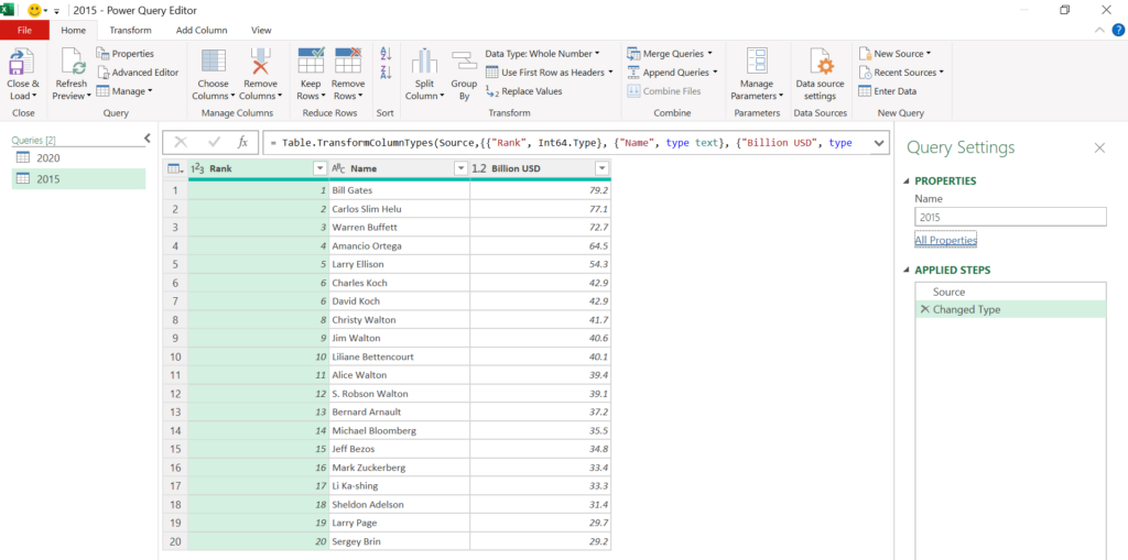
Table will get loaded into the Power Query Editor.
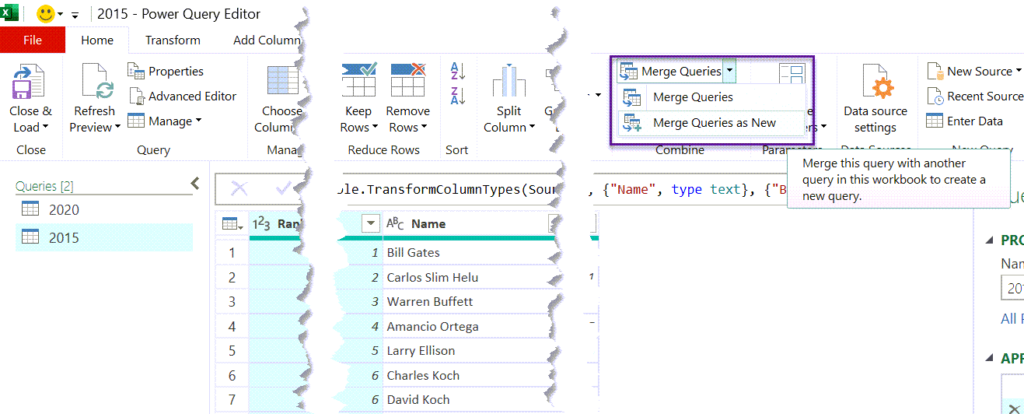
Once both Tables are loaded, we can use the different Merge options in Power Query to find the common records between the tables. For that go to the Home tab of the Power Query Editor > Merge Queries > Merge Queries as New
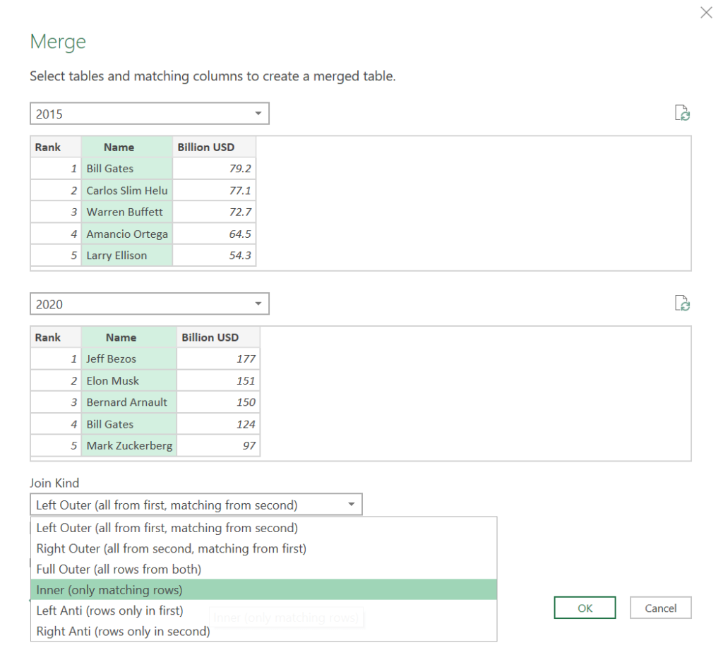
A dialog called Merge will be activated. Select the tables to merge using the Drop Down List and click on the columns containing Values to compare (Colum called Name in this case) in both tables.
Next step is to specify the Join Kind.
Power Query provides 6 types of Joins for merging tables, out of which Inner Join is used to find matching records. We want common records between both tables, so select Inner Join and click on OK.
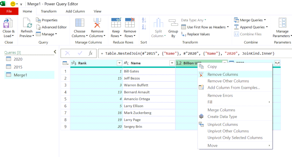
And we have a new table containing the common Values. To remove the unwanted columns, right click on the column header and select Remove columns.
Rename the column header if you want to. Here I have renamed the column as Common Names.
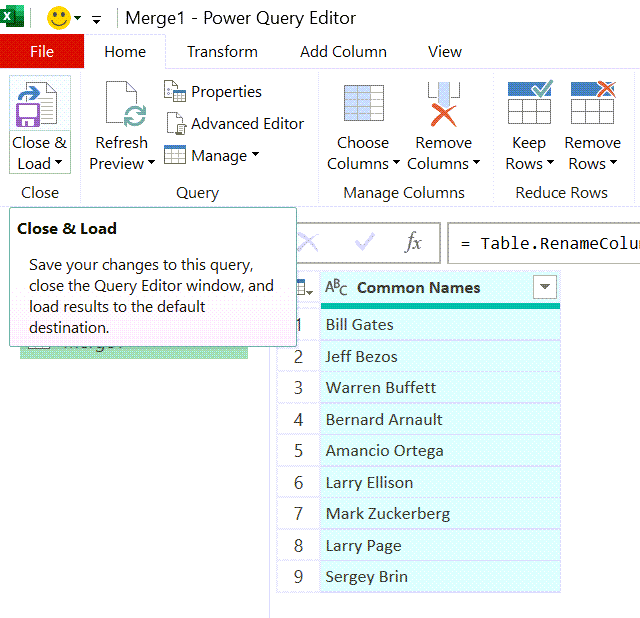
Click on Close & Load in the Home tab the Power Query Editor and the above table, i.e., the table containing common values between 2 List of Billionaires will be loaded into a new Excel Worksheet.