In this tutorial, I will show you 5 different ways to Extract only Numbers from a list of Strings.
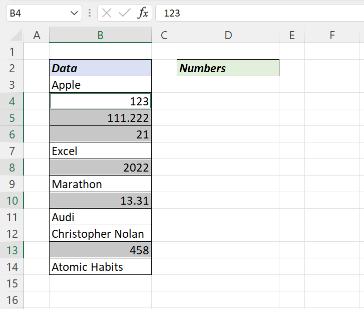
Following is a Table containing Text as well as Numeric Values and we will be using this data for explaining the different methods.
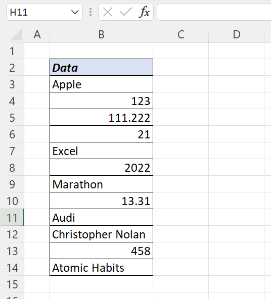
Table of Contents
FILTER Function to extract Numbers
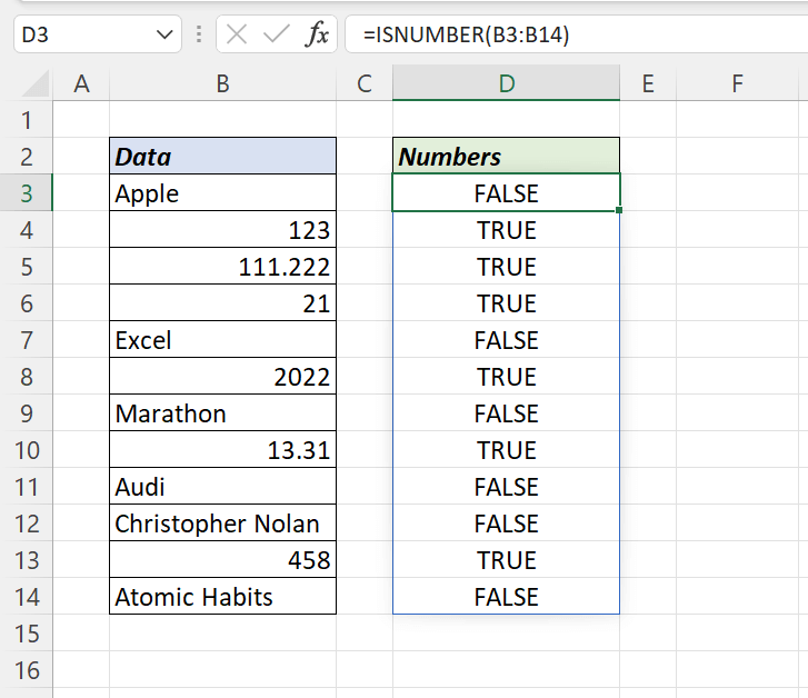
The ISNUMBER function in Excel can be used to check whether a string is a Number or Text.
When a string is supplied into the ISNUMBER function, the function will return TRUE, if it’s a Number.
And FALSE, if the string is a Text.
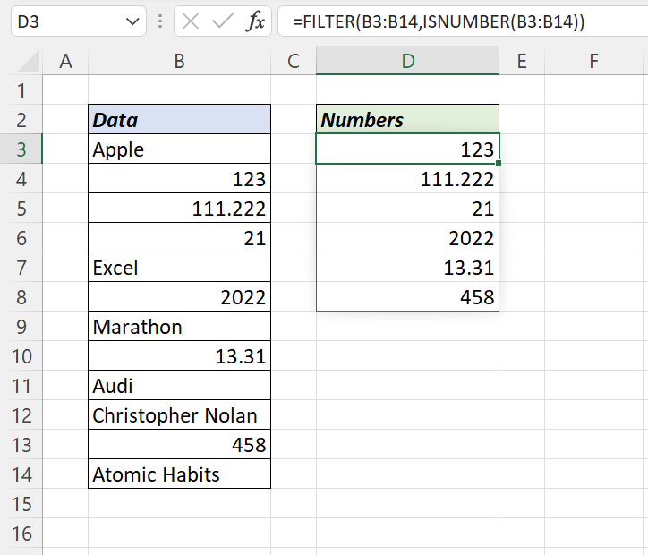
These TRUE and FALSE values can be used inside the FILTER function to extract only numbers.
The following formula will return the numeric values in the range B3:B14
=FILTER(B3:B14,ISNUMBER(B3:B14))
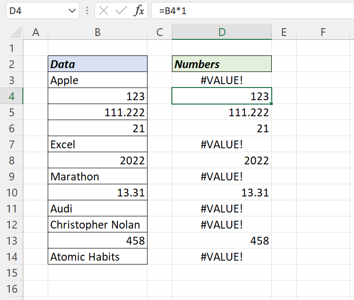
Arithmetic operation to extract Numbers
When we multiply a string with the value 1, the result will be the string itself, if the string is a numeric value.
If the string is a text value, the formula will return #VALUE! error.
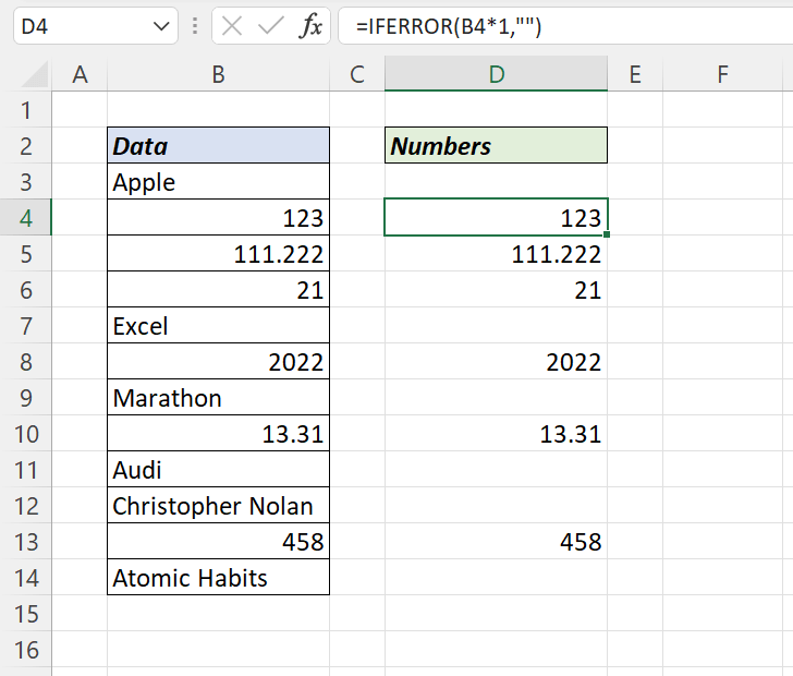
The IFERROR function in Excel is then used to get rid of the Error values.
=IFERROR(B4*1,"")
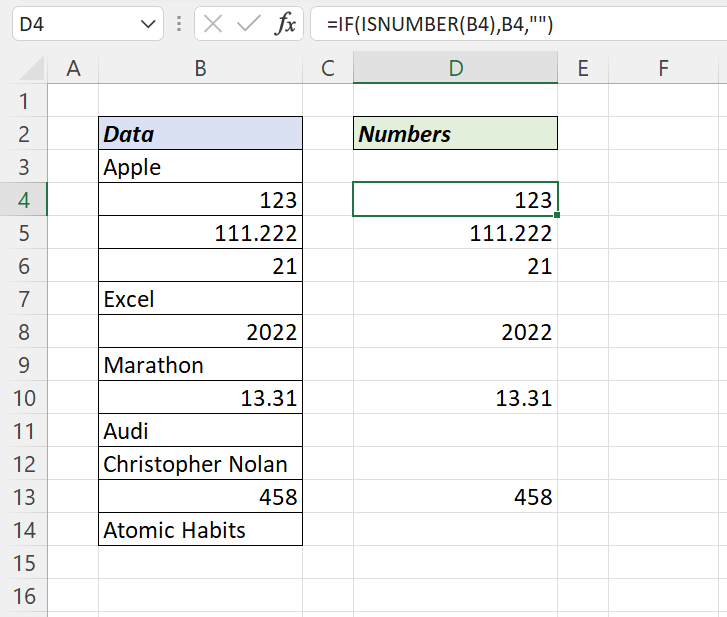
Combination of IF and ISNUMBER Function to extract Numbers
In the following formula, ISNUMBER function is used check whether the string is a Number or not.
The IF function will use this result and return the string itself for TRUE and a Null value for FALSE.
=IF(ISNUMBER(B4),B4,"")
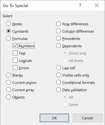
Go To Special to extract Numbers
The Go To Special option in Excel can be used to select cells, containing Numbers, Formulas, Errors, etc.,
To extract the numbers from a data range,
select the data range > press Ctrl + G to activate the Go To dialog
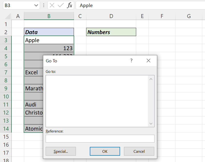
Click on Special… to activate the Go To Special dialog.
Select Constants > mark the check box for Numbers and click on OK
All those cells containing numbers are selected. Press Ctrl + C to copy the cells.
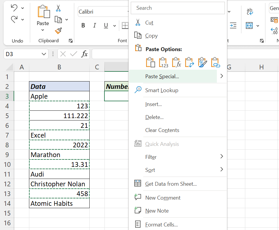
Right-click on the cell where you want to paste it and click on the first option listed under Paste Options:
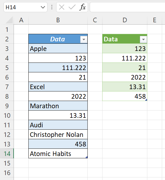
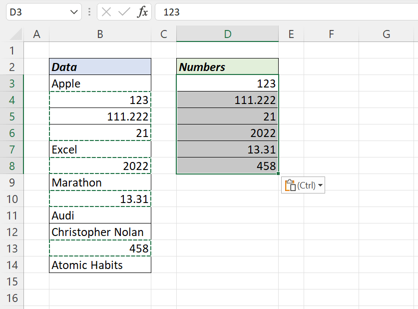
And we have extracted the numeric values present in the table.
Power Query to extract Numbers
To load the table into Power Query Editor of Excel,
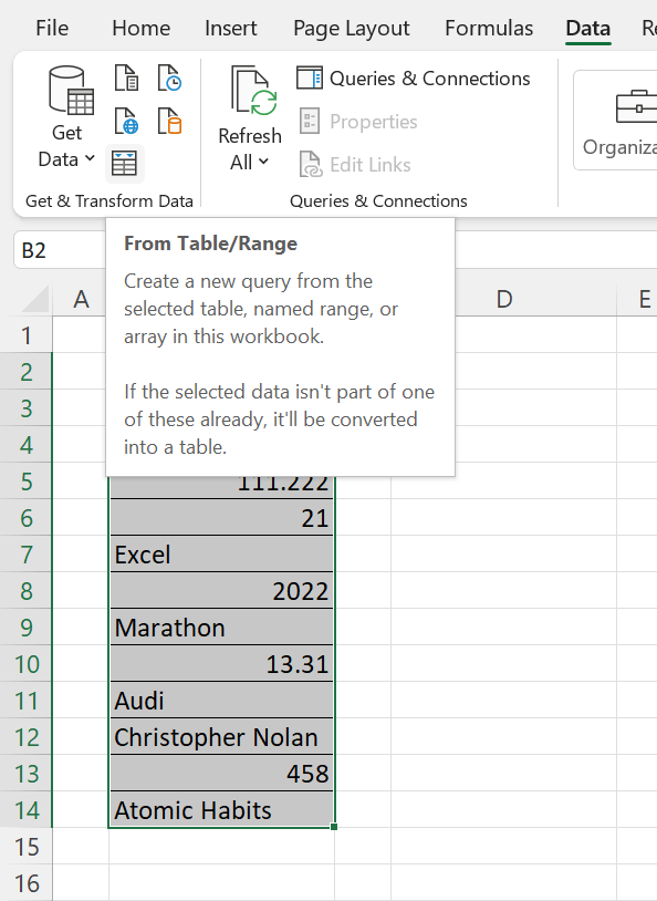
Select the table > go to the Data tab of the Excel Ribbon > From Table/Range
If the data range is not an official Excel Table, we will be prompted to convert the data range into a Table
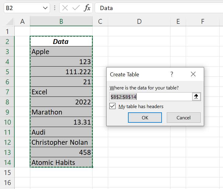
Once you click on OK in the Create Table dialog, the table will be loaded into the Power Query editor of Excel
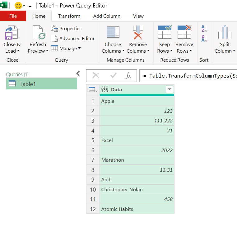
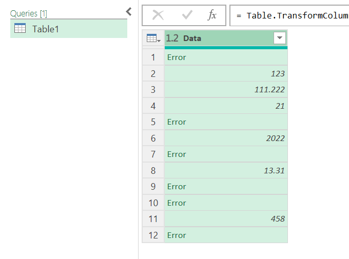
In this method, the trick is to apply Decimal Number data type to the column.
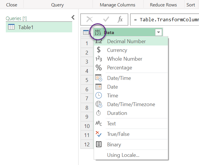
For that, click on the icon ABC123 on the left side of the column header and select Decimal Number.
All those cells with text values will display an Error.
To remove the rows containing Error, right-click on the column header and select Remove Errors.
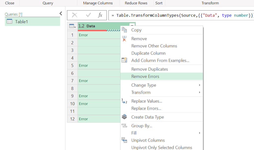
Errors are all gone and the rows with numbers remain.
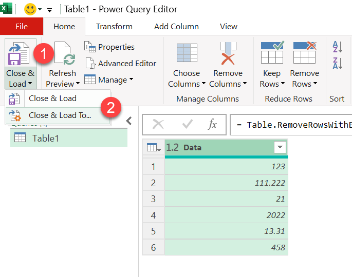
To load this data into the Excel worksheet, click on the split button called Close & Load > Close & Load To…
Import Data dialog is activated. Click on the radio button for Existing worksheet and specify the cell where we want to insert the output table.
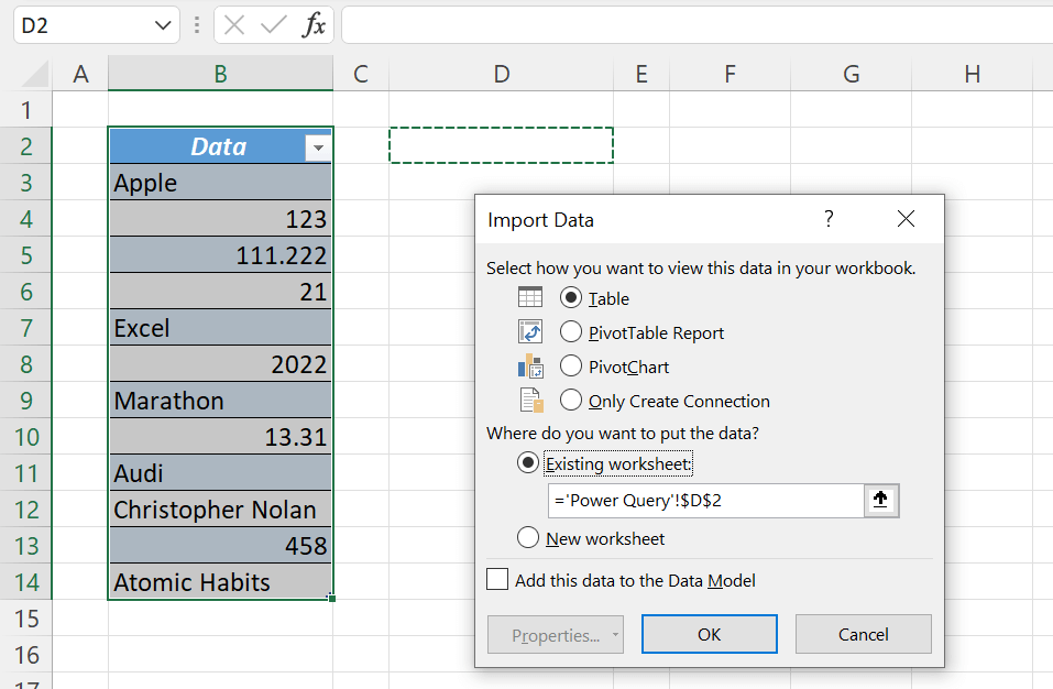
Click OK and we have a new table containing numbers extracted from the source table.