To put a list or table in random order, for quiz questions, a random draw or a fair rota, use =SORTBY(A2:C20,RANDARRAY(ROWS(A2:C20))) in Excel 365. In any version, a RAND helper column and a sort does the same.
Excel 365SORTBY + RANDARRAY
Any versionRAND column + Sort
New orderPress F9
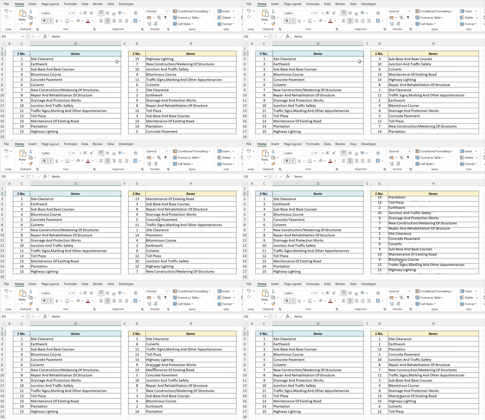
Method 1: SORTBY and RANDARRAY (Excel 365)
=SORTBY(B3:D17,RANDARRAY(ROWS(B3:D17)))RANDARRAY gives each row a random number, and SORTBY orders the rows by them. Press F9 for a new order. The original data isn't touched.
Method 2: RAND column and sort (any version)
- Insert a column next to the data and fill it with
=RAND(). - Click any cell in that column → Data → Sort Smallest to Largest.
- Delete the RAND column if you don't need it any more.
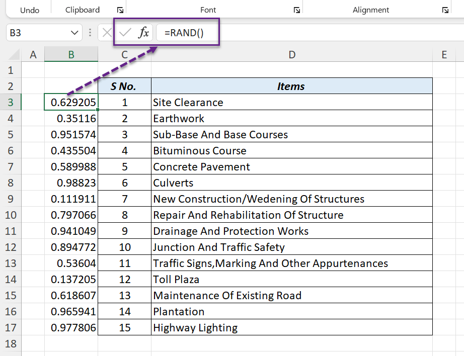
This rearranges the original rows, so keep a copy if the order matters.
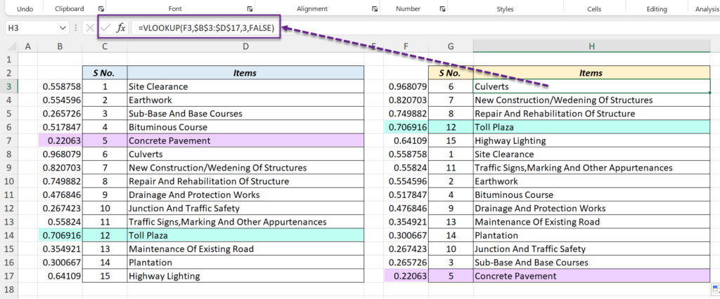
Method 3: Formulas that keep the original (any version)
With RAND values in B3:B17, list them largest first:
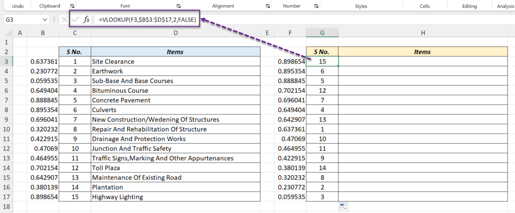
=LARGE($B$3:$B$17,ROWS($B$3:B3))Then look up each row's record by its random number:
=VLOOKUP(F3,$B$3:$D$17,2,FALSE)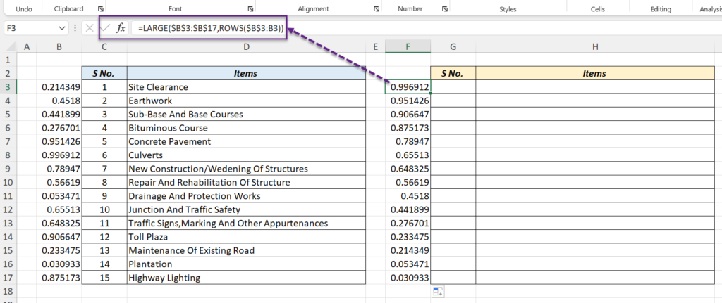
Things to know
- RAND and RANDARRAY recalculate after every edit, so the order keeps changing. To keep one shuffle, copy the result and Paste Special → Values.
- To pick just a few random rows, wrap Method 1 in TAKE:
=TAKE(SORTBY(B3:D17,RANDARRAY(ROWS(B3:D17))),5). - For one random item, see pick a random value from a list.