Why Unpivot or Normalize Data?
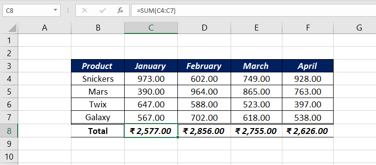
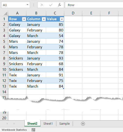
Data in a Report format may give you the insight of a particular aspect, but that report need not be good for further analysis or generating another report or reports. Following is a sample data in Report format.
It is always easy to Filter, Sort, Slice or Dice data, when all the values of the same type are in a single column.
Suppose you want to filter the sales amount of a particular product for a month or two, it almost impossible to do that with a report like this.
Moreover, Pivot Tables also are not friendly to data in report format.
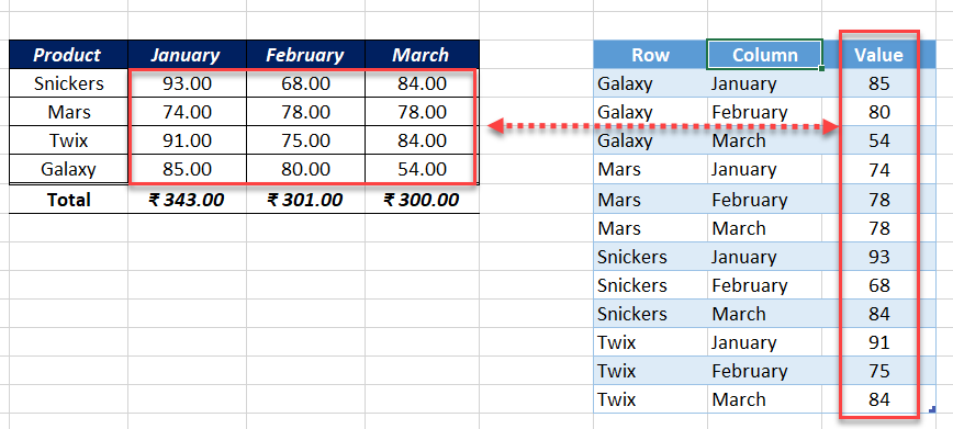
Now, see the data on right side of the image below. It is the normalized form of the data on left.
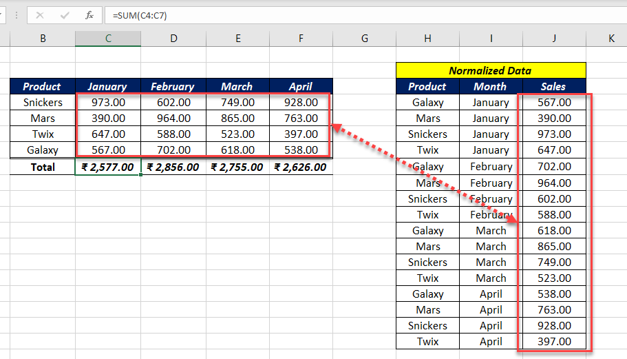
As you can see, sorting and filtering are easy with Normalized data.
The basic rule of DataStructure is that all the values of the same type should be in one column.
How to convert the Data in a Report format into it’s simplest form which is suitable for further Analysis or Creating Pivot Table Reports is explained in this article. The process is known in different names like Normalization of Data, UnPivoting Data, Reverse Pivoting Data etc.
How to UnPivot or Normalize data
Here, I will be using PivotTable & PivotChart Wizard for UnPivoting Data. The same process done using Power Query is explained in the following article. How to Unpivot Data using Power Query
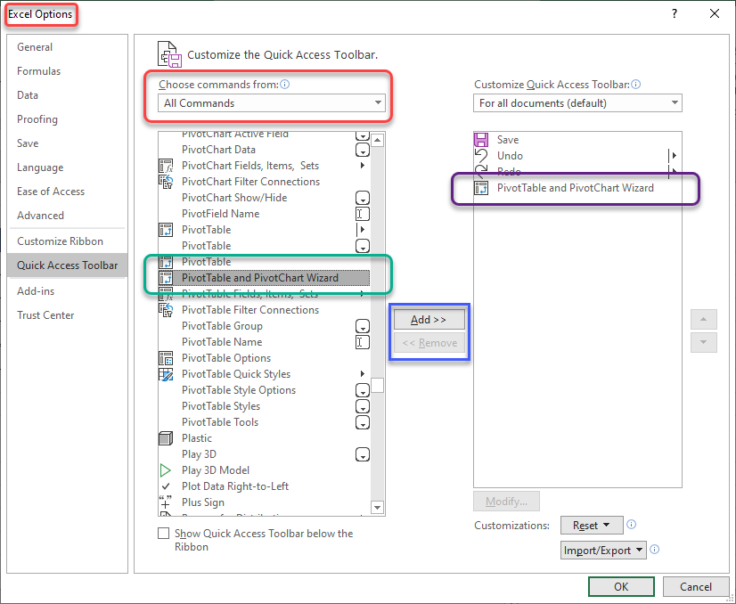
By default, PivotTable & PivotChart Wizard won’t be available in the Excel Ribbon or Quick Access Toolbar. So, we need to manually add this option to the QAT. To add PivotTable and PivotChart Wizard to Quick Access Toolbar,
Right-click on QAT > Customize Quick Access Toolbar… > In the Excel Options dialog box > Select All Commands from the drop-down menu under Choose commands from > Select PivotTable and PivotChart Wizard from the list > Click on Add > Click OK
You can also use the shortcut ALT + D + P to activate PivotTable and PivotChart Wizard.
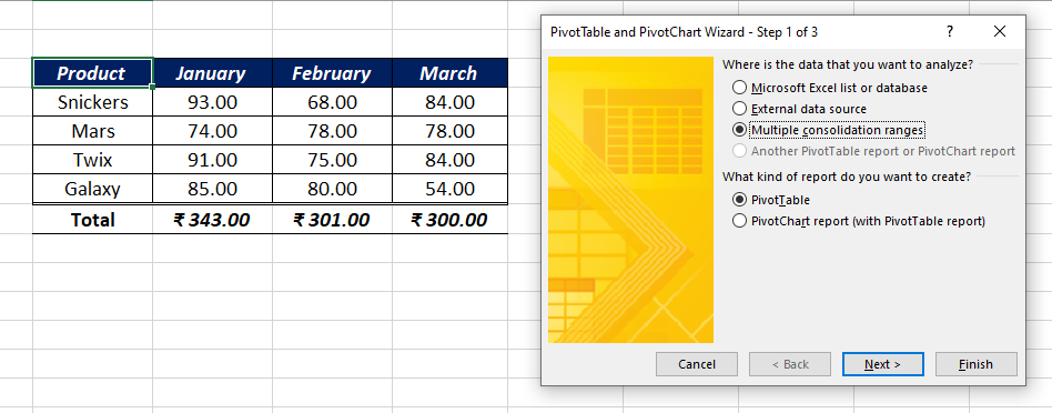
Once the PivotTable and PivotChart Wizard is activated, Select the radio button against Multiple consolidation ranges and Click on Next
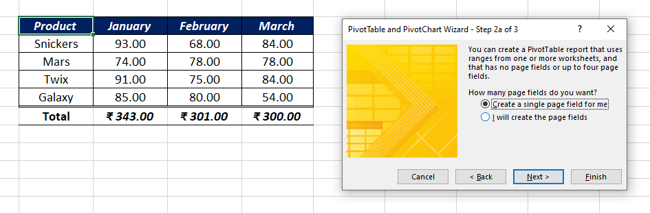
Select I will create the page fields and Click on Next
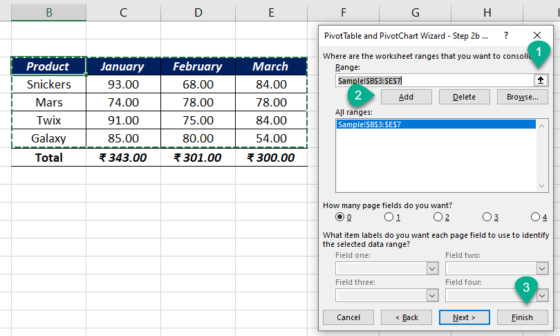
Click on the up arrow under the label called Range (1) > Select the range of cells containing data > Click on Add (2) > Finish (3)
A new worksheet will be created with a Pivot Table like the following.
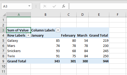
Double click on the Grand Total value (the cell containing the value 944) and a new worksheet will be created with all those records that has constituted to this value.
By double clicking on a value in the Pivot Table report, we are making using of the drill-down option of Pivot Tables.
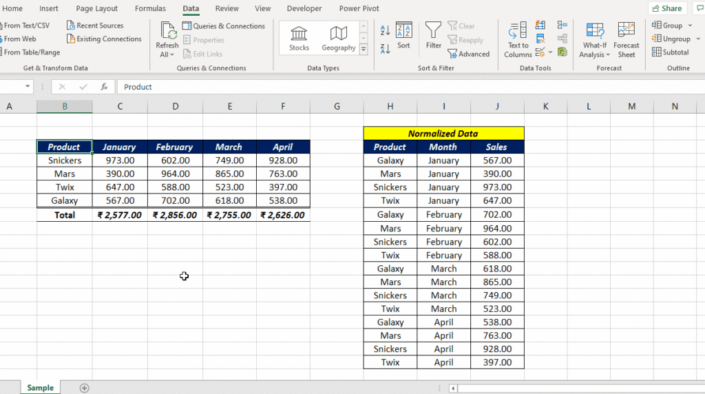
This data is the normalized form of the data which we have in the Report form.
To UnPivot data using Power Query, read the following article.