Remove or Extract Special Characters from a data set using Power Query

In this article, I will explain an easy method to Extract or Remove Special Characters, Alphabets or Numerals from a data set using Power Query in Excel.

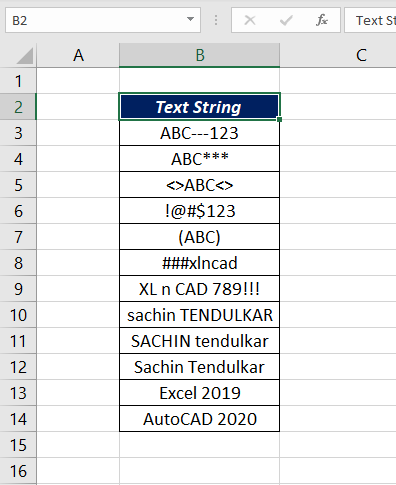
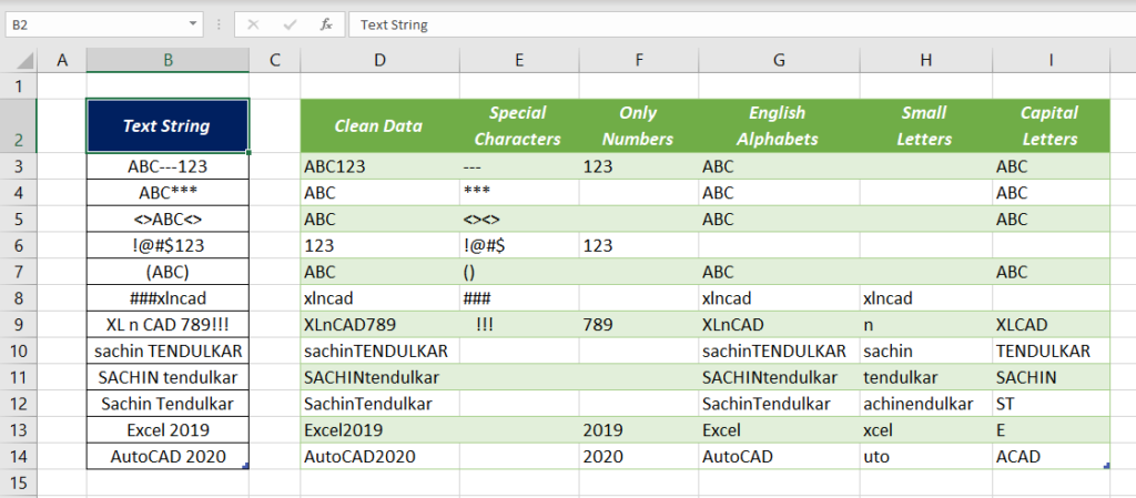
Following is the data set from which I want to remove the special characters like ‘!’, ‘@’, ‘#’, ‘$’, ‘%’, ‘&’, ‘*’, ‘(‘ etc.

To clean this data, i.e. to remove the special characters,

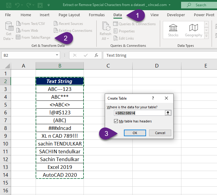
Select a cell in the data set > Data tab > From Table/Range > Click OK in the dialog called Create Table

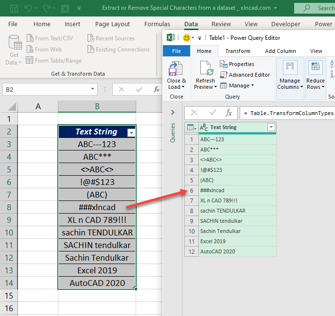
Selected data is loaded into the Power Query Editor.

To create a new column containing the same data without special characters, go to the Add Column tab of Power Query Editor > Click on Custom Column

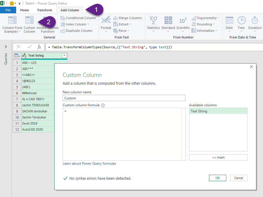
In the Custom Column dialog, type in the name for the New column. Here, I have used Clean Data as the New column name.

Now, the formula to remove special characters.

=Text.Select([Text String],{"A".."z","0".."9"})

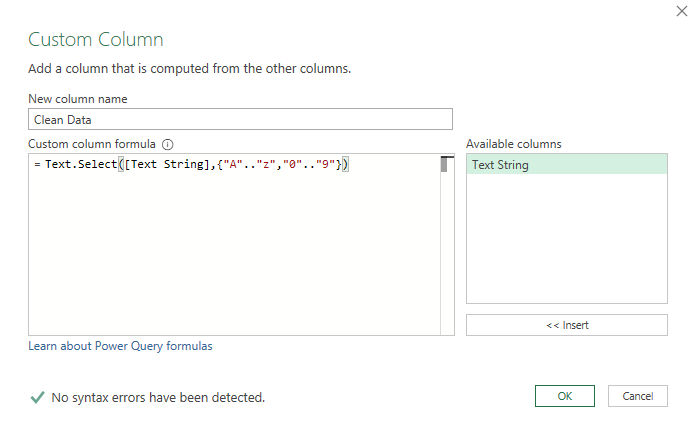
Text.Select is a M function which will extract the ‘type of characters’ specified inside the function and Text String is the column containing data.

In fact, we are not removing special characters, but extracting the characters such A, B, C, … X, Y, Z, a, b, c, up to x, y, z and the numbers from 0, 1, 2, up to 9.

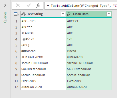
When I click OK, we have a new column called Clean Data which contains the data without special characters.

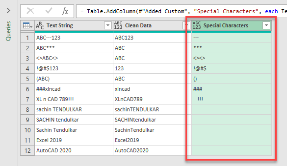
Now, If you want to extract the special characters from the same data, use the following formula.

=Text.Remove([Text String],{"A".."z","0".."9"})

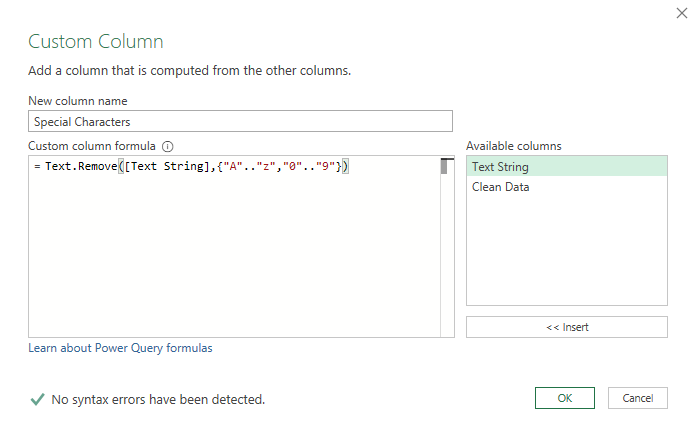
Text.Remove is a M function which will remove the characters specified inside the function.

A new column called Special Characters is created, which contains only the special characters is created.

Now, that we know what Text.Remove and Text.Select functions does, let’s explore the different possibilities of these two functions.

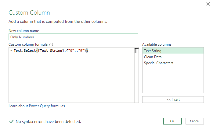
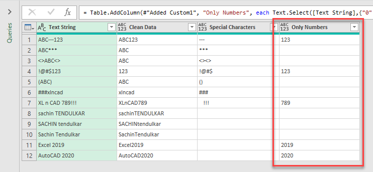
To extract only the numbers from the same data, use the following formula.

=Text.Select([Text String],{"0".."9"})

Another column called Only Numbers which contains only the numbers is created.

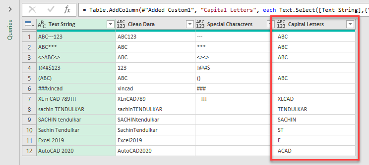
To extract only the letters that are in Upper Case,

=Text.Select([Text String],{"A".."Z"})

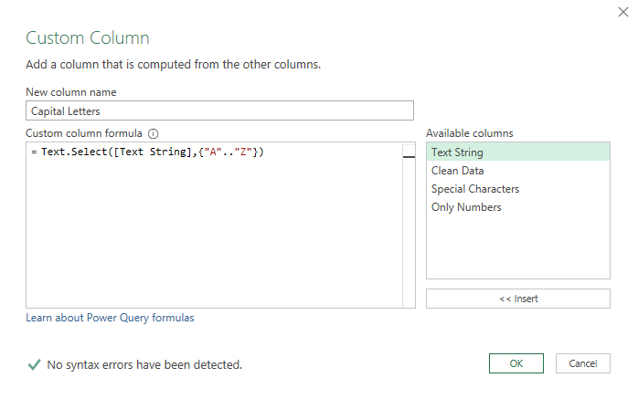
A new column called Capital Letters which contains only Capital Letters is created.

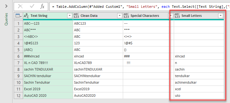
To extract only the letters that are in Lower Case,

=Text.Select([Text String],{"a".."z"})

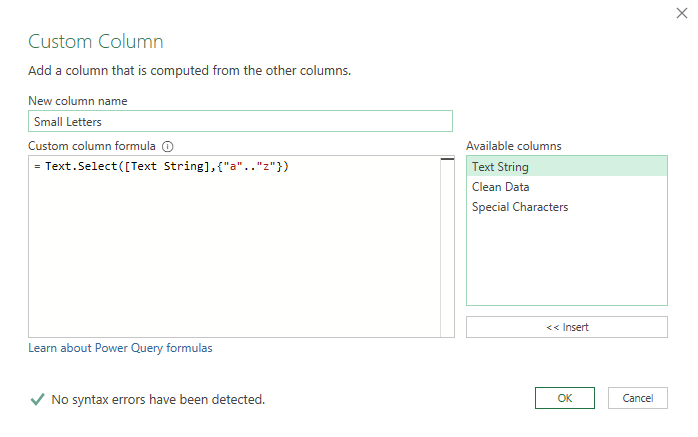
A new column called Small Letters which contains only the lower cases letters is created.

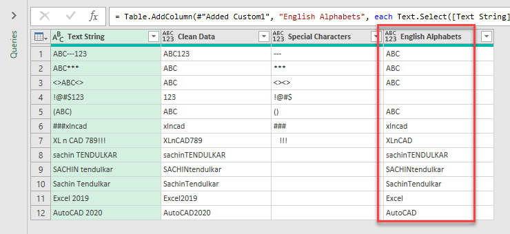
To extract all the English Alphabets,

=Text.Select([Text String],{"a".."z","A".."Z"})

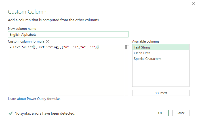
We have a new column called English Alphabets which contains only English alphabets, both Capital and Small letters.

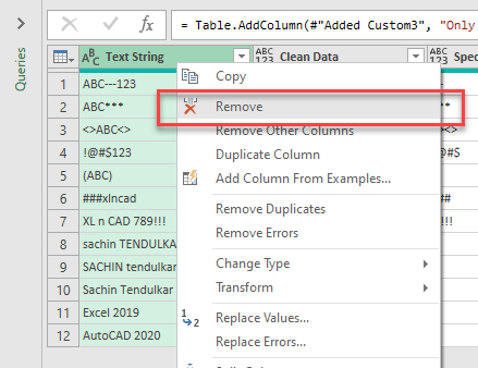
To remove a particular column, right-click on the column header and select Remove.

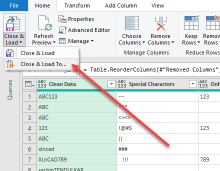
To load this data into the Excel sheet, Click on the split button for Close & Load in the Home tab of the Power Query Editor > Close & Load To…

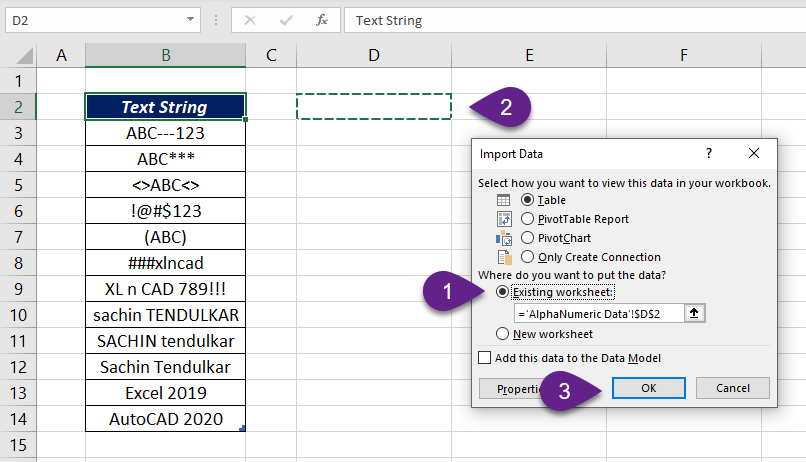
In the Import Data dialog > Select Existing worksheet > Select the cell where you want to place the data and Click OK

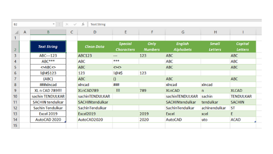
Here, we have a table with different columns containing, ‘data without special characters’, ‘only special characters’, ‘only numbers’, ‘English alphabets’, ‘English alphabets in Lower Case’ and ‘English alphabets in Upper Case’.